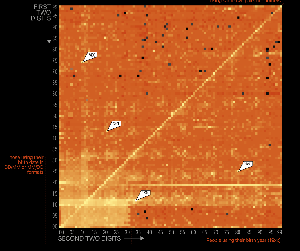
13 years ago, Pr. Michio Kaku, a renowned physicist, professor at Stanford, explained that USA’s secret weapon was “The genius visa” (H1-B), a Visa that allows exceptional scientists to migrate to the US. It’s the key to compensate for the failure of the American educational system. Is it also the case for AI?
Dr Laurent Alexandre (the founder of Doctissimo) seemed to think alike, as in 2017, during a presentation in front of the French Senat, he explained that Artificial Intelligence was developed using non-American brains, European and American data but by and for American companies.
So, in 2025, is it true? Did we lose our AI Geniuses to the USA?
In 2023, AI Magazine made a Top 10 of AI Leaders.

For these 10 AI leaders, here are some very self explaining figures:


As you can see, they all work for American companies while 9 out of then are born elsewhere and 7 out of 10 have been educated outside of USA. 5 out of 10 comes from Europe.
For scientific accuracy, Demis Hassabis works in UK for DeepMind, a UK company acquired by Google to boost their AI development progress, but is considered as working for an American company as all the benefits of his work go to Google.
So, what should we change to keep our brilliant minds?
Here is the Jupyter Notebook with the data and the code used to create the 3 maps:
# Import all necessary libraries
import matplotlib.pyplot as plt
import cartopy.crs as ccrs
import cartopy.feature as cfeature
from collections import defaultdict
# Data for each category with approximate coordinates
birth_data = {
"Andrew Ng": {"country": "UK", "lat": 51.5, "lon": -0.1278},
"Fei-Fei Li": {"country": "China", "lat": 39.9042, "lon": 116.4074},
"Andrej Karpathy": {"country": "Slovakia", "lat": 48.1486, "lon": 17.1077},
"Demis Hassabis": {"country": "UK", "lat": 51.5, "lon": -0.1278},
"Ian Goodfellow": {"country": "USA", "lat": 37.7749, "lon": -122.4194},
"Yann LeCun": {"country": "France", "lat": 48.8566, "lon": 2.3522},
"Jeremy Howard": {"country": "Australia", "lat": -33.8688, "lon": 151.2093},
"Ruslan Salakhutdinov": {"country": "Russia", "lat": 55.7558, "lon": 37.6173},
"Geoffrey Hinton": {"country": "UK", "lat": 51.5, "lon": -0.1278},
"Alex Smola": {"country": "Germany", "lat": 52.5200, "lon": 13.4050}
}
first_degree_data = {
"Andrew Ng": {"country": "USA", "lat": 40.4406, "lon": -79.9959},
"Fei-Fei Li": {"country": "USA", "lat": 40.3430, "lon": -74.6514},
"Andrej Karpathy": {"country": "Canada", "lat": 43.6532, "lon": -79.3832},
"Demis Hassabis": {"country": "UK", "lat": 52.2053, "lon": 0.1218},
"Ian Goodfellow": {"country": "USA", "lat": 37.4275, "lon": -122.1697},
"Yann LeCun": {"country": "France", "lat": 48.8566, "lon": 2.3522},
"Jeremy Howard": {"country": "Australia", "lat": -37.8136, "lon": 144.9631},
"Ruslan Salakhutdinov": {"country": "Russia", "lat": 55.9160, "lon": 37.4160},
"Geoffrey Hinton": {"country": "UK", "lat": 52.2053, "lon": 0.1218},
"Alex Smola": {"country": "Germany", "lat": 52.5200, "lon": 13.4050}
}
working_data = {
"Andrew Ng": {"country": "USA", "lat": 37.7749, "lon": -122.4194}, # e.g. Coursera/Landing AI
"Fei-Fei Li": {"country": "USA", "lat": 37.4275, "lon": -122.1697}, # Stanford affiliated companies, USA
"Andrej Karpathy": {"country": "USA", "lat": 37.4419, "lon": -122.1430}, # Tesla (USA)
"Demis Hassabis": {"country": "USA", "lat": 37.422, "lon": -122.084}, # DeepMind (UK) - Owned by Google (USA)
"Ian Goodfellow": {"country": "USA", "lat": 37.7749, "lon": -122.4194}, # Google (USA)
"Yann LeCun": {"country": "USA", "lat": 40.7128, "lon": -74.0060}, # Meta/Facebook (USA)
"Jeremy Howard": {"country": "USA", "lat": 37.7749, "lon": -122.4194}, # fast.ai (USA)
"Ruslan Salakhutdinov": {"country": "USA", "lat": 40.4406, "lon": -79.9959}, # Carnegie Mellon (USA)
"Geoffrey Hinton": {"country": "USA", "lat": 37.422, "lon": -122.084}, # Google (USA)
"Alex Smola": {"country": "USA", "lat": 47.6062, "lon": -122.3321} # AWS (USA)
}
# Functions definition
def aggregate_data(data):
"""
Aggregate the data by country.
Returns a dictionary mapping country to a dict with keys:
- count: number of entries for that country,
- lat: average latitude,
- lon: average longitude.
"""
aggregated = defaultdict(lambda: {"count": 0, "sum_lat": 0, "sum_lon": 0})
for person, info in data.items():
country = info["country"]
aggregated[country]["count"] += 1
aggregated[country]["sum_lat"] += info["lat"]
aggregated[country]["sum_lon"] += info["lon"]
# Compute the average for each country
for country in aggregated:
count = aggregated[country]["count"]
aggregated[country]["lat"] = aggregated[country]["sum_lat"] / count
aggregated[country]["lon"] = aggregated[country]["sum_lon"] / count
# Remove the temporary sum values
del aggregated[country]["sum_lat"]
del aggregated[country]["sum_lon"]
return aggregated
def plot_aggregated_world_map(aggregated_data, title, offsets, default_offset=(20, 20), base_size=50, size_increment=50):
"""
Plots the aggregated map with country-specific offsets.
Parameters:
- aggregated_data: dict, aggregated data from aggregate_data()
- title: str, title of the plot.
- offsets: dict, mapping country names to (dx, dy) offsets.
- default_offset: tuple, offset to use for countries not specified in offsets.
- base_size: int, base marker size.
- size_increment: int, additional marker size per extra individual.
"""
fig = plt.figure(figsize=(10, 5))
ax = plt.axes(projection=ccrs.PlateCarree())
ax.set_global()
ax.coastlines()
ax.add_feature(cfeature.BORDERS, linestyle=':')
ax.add_feature(cfeature.LAND, facecolor='#C2E812')
ax.add_feature(cfeature.OCEAN, facecolor='#84D2F6')
for country, info in aggregated_data.items():
count = info["count"]
lat = info["lat"]
lon = info["lon"]
marker_size = base_size + (count - 1) * size_increment / 2
plt.plot(lon, lat, marker='o', color='#467082', markersize=marker_size/5, transform=ccrs.PlateCarree())
# Get the offset for this country or use the default
dx, dy = offsets.get(country, default_offset)
ax.annotate(f"{country} ({count})",
xy=(lon, lat),
xycoords=ccrs.PlateCarree()._as_mpl_transform(ax),
xytext=(lon+dx, lat+dy),
textcoords=ccrs.PlateCarree()._as_mpl_transform(ax),
arrowprops=dict(arrowstyle="->", color='black', lw=0.5),
fontsize=12,
bbox=dict(boxstyle="round,pad=0.3", fc="white", alpha=0.9))
plt.title(title)
plt.show()
# Define offset per country for better visualisation
country_offsets = {
"UK": (-20, 20),
"China": (-20, 30),
"Slovakia": (30, -20),
"USA": (20, -20),
"France": (-50, 0),
"Australia": (-40, 10),
"Russia": (10, 10),
"Canada": (0, 20),
"Germany": (-40, -20)
}
# Aggregate data for each category
agg_birth = aggregate_data(birth_data)
agg_first_degree = aggregate_data(first_degree_data)
agg_working = aggregate_data(working_data)
# Plot the aggregated maps using country-specific offsets
plot_aggregated_world_map(agg_birth, "Birthplaces of Top Ten AI Scientists, aggregated by Country", country_offsets)
plot_aggregated_world_map(agg_first_degree, "First University degree's locations of Top Ten AI Scientists, aggregated by Country", country_offsets)
plot_aggregated_world_map(agg_working, "Current Working Places of Top Ten AI Scientists, aggregated by Country", country_offsets)